Activation steering

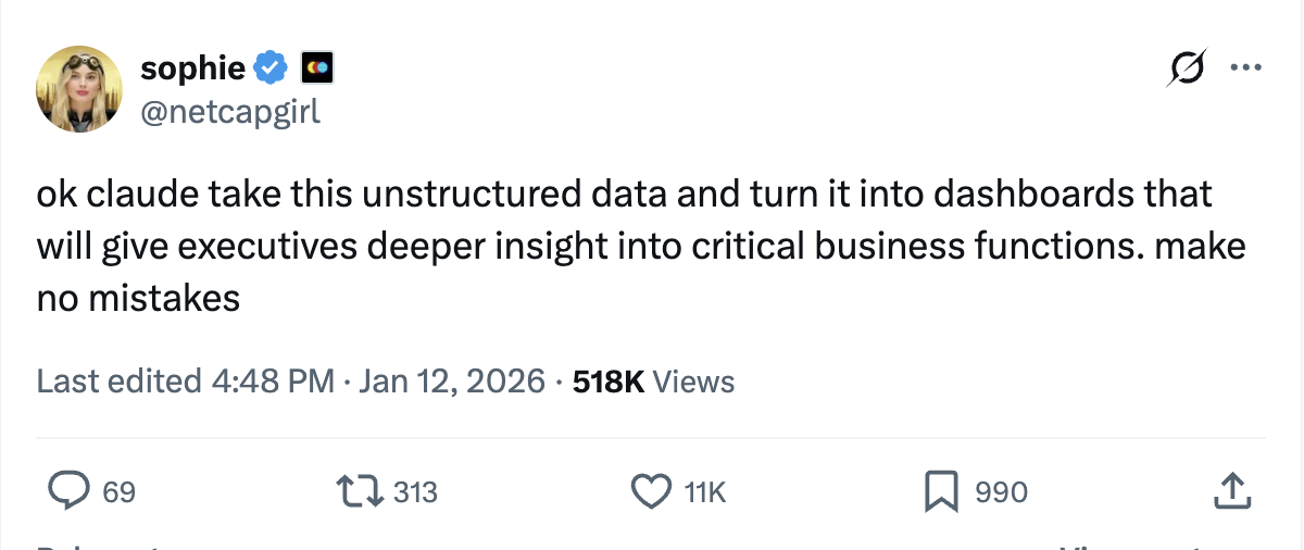
What do you do when you want a chatbot to change something about the responses it’s been giving you? The natural tactic is to simply tell it (prompt it). “No - make it less formal.” “Write from a legal assistant’s point of view.” Or, the very well-known, “make no mistakes”:

However, there exists a way to do this from the inside of the model as well, known as representation engineering (RepE). In this post, I’ll describe the basics of RepE as well as some examples of where it can be deployed.

Introduction

The main idea behind RepE is fairly intuitive: first, find a vector representing the ‘direction’ you want to guide the model towards (for example, a more formal writing style). Then at inference time, add that vector to the model’s hidden states.

(Note: Inference in Machine Learning is the stage at which you use the already trained model to generate your response. For example, when you ask ChatGPT, “Please solve this homework question for me,” ChatGPT reads in your response token-by-token, computes some output logits, and converts them into tokens to provide you with your homework answer. It’s different from the training stage, which actually updates the model weights to help the model learn.)

However, there are lots of ways to change a model’s behavior. How does representation engineering differ from finetuning, which also deals with the “inside” of the model? How does it differ from prompting, which is also an inference-time method? Below is a simple guide.

Personally, RepE interests me because it directly deals with the internals of the model. You’re basically going ‘inside’ and getting your hands dirty. Finetuning and prompting can be effective methods for changing a model’s behavior, but can have less fine-grained control over their outcomes. Regardless, all three general methods have their place depending on the type of problem being solved.

So, how does all of it work? RepE works thanks to a model’s residual steam. Let’s take a closer look at the transformer architecture to see where exactly RepE makes its edits.

How the transformer works

Suppose we give the LLM the following message:

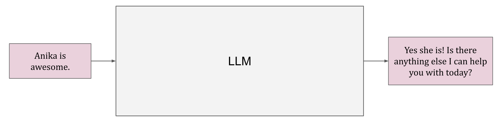
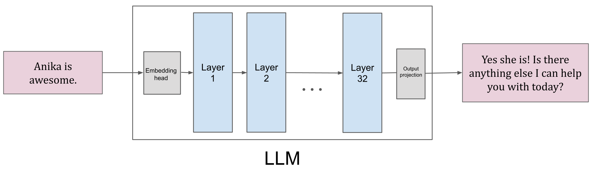
What goes on inside? Well, modern-day language models are composed of different layers, or transformer blocks. In this example, let’s suppose there are 32 layers within the model.

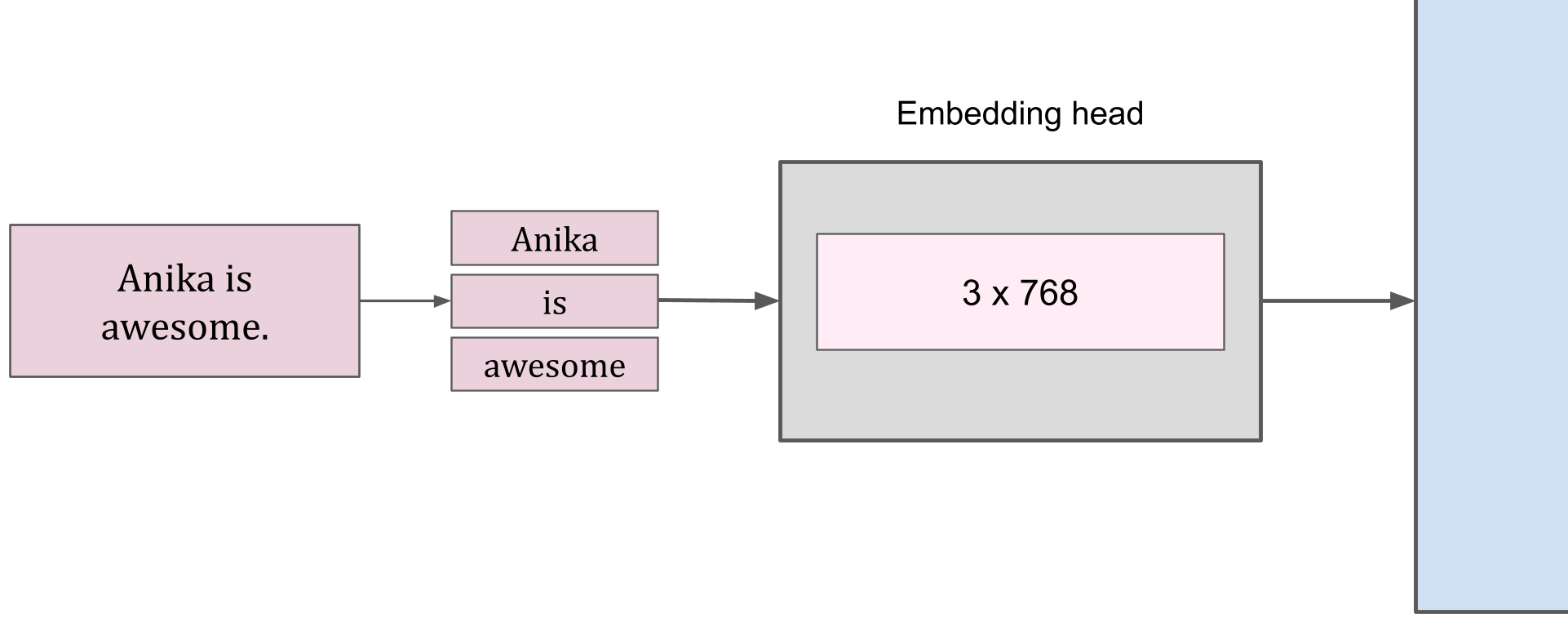
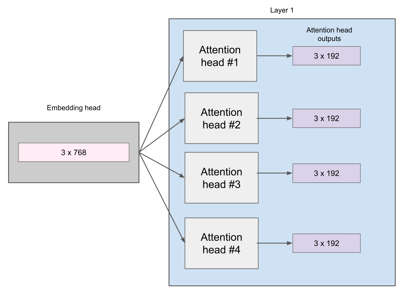
First, let’s begin with the embedding dimension. The model reads in token-by-token. Assuming “Anika is awesome” gets broken up into 3 tokens, and each word embedding has 768 dimensions, then after applying the embedding step, we get a resulting 3x768 matrix.

Next, we pass in the embedded message to the first layer. We can pretend that the first layer has 4 attention heads, which each play varying roles in finding patterns in different parts of the text. Each attention head performs some matrix multiplication calculations (with its learned query, key, and value weight matrices) and results in four separate attention head vectors.

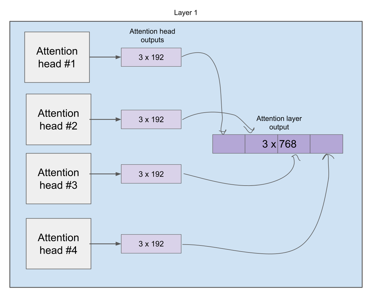
Next, we concatenate the four attention head vectors into one and apply a learned linear output projection matrix to mix information across heads.

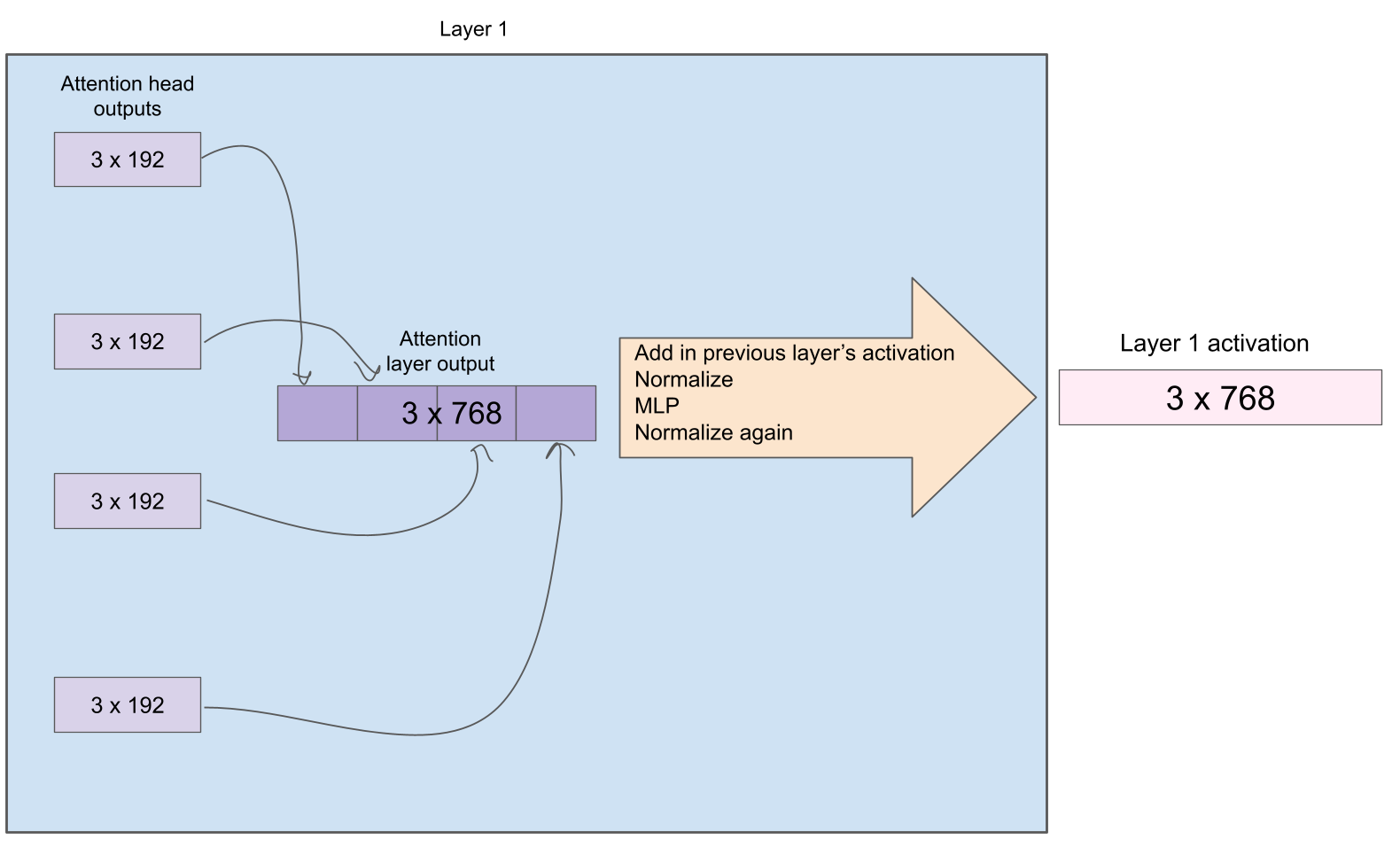
Finally, after conducting a few more steps (adding in the previous layer’s activation (in this case, the embedding), normalizing, applying the MLP transformation, and normalizing again), we obtain the final hidden state for the first layer.

Then, we place this activation back into Layer 2, repeat the whole process, and then Layer 3, and then repeat the whole process… until we get to the very last layer. After all these transformations and computations, the last layer’s activation is what is used to predict the next token of the LLM’s response in the output head.

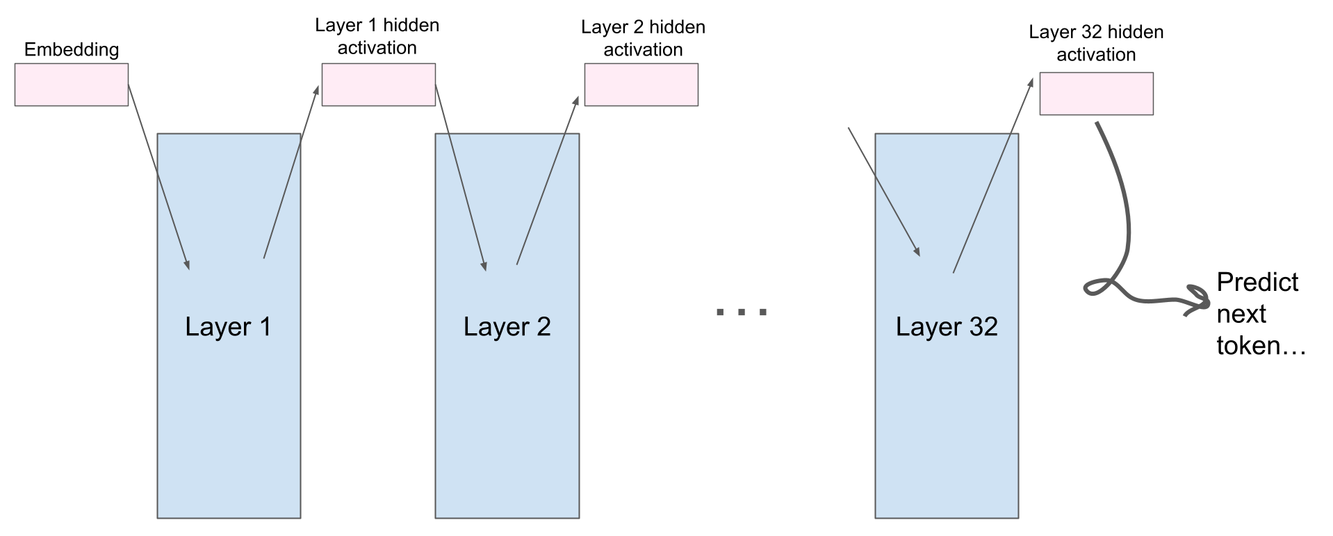
At first glance, the hidden activations (the pink blocks) don’t seem to be that special. They are each simply input for their respective next layer. However, RepE researchers found that these very hidden dimensions can be manipulated to steer a model’s entire behavior! As a whole, these activations are what make up the residual stream of the transformer. Like a stream, these hidden activations ‘flow’ through the model, undergoing computations until they reach the last layer, where they are used to predict the next token.

Finding the steering vector

Earlier, I mentioned that to change the behavior of the model, you first find a vector representing the ‘direction’ you want to guide the model towards, and then add that vector to the model’s residual stream. But how do you even find this vector in the first place? A common method is contrastive pairing.

The main idea behind contrastive pairing is fairly intuitive: subtract the behavior that you don’t want from the behavior that you do want. For example, suppose you want your LLM to be more optimistic. First, you would collect a set of prompts that contain optimistic responses. This would be your positive set. Next, you collect your negative set, which would be a set of texts that contains pessimistic responses.

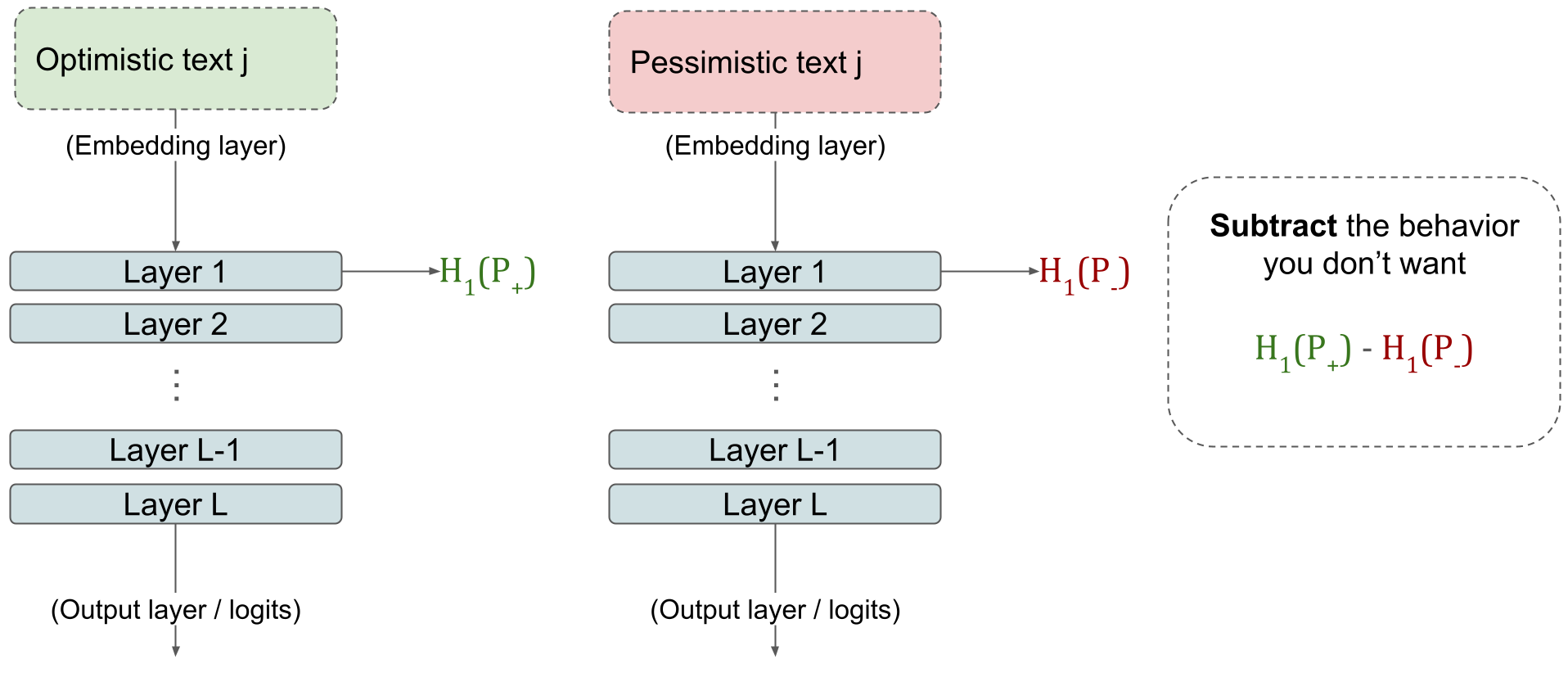
For each pair of texts j, (1) pass each one through the model, (2) extract the hidden states at a specific layer, and (3) simply subtract the activation of your negative set from your positive set. Repeat across all prompts and average out the subtractions to obtain your final steering vector that will ‘push’ the model to produce more optimistic responses.

(Another variation instead of averaging out the subtractions is to use PCA to find the vector that has the highest variation. The idea is that this vector holds information about the largest ‘difference’ between positive and negative sets. As you can see, there are plenty of methods and variations to find your ideal steering vector.)

Something I find really exciting about steering vectors is that you don’t need a lot of data to find the correct one. Modern methods often use fewer than 100 examples, whereas fine-tuning requires thousands and thousands of data samples. This is pretty neat, because it means you can hand-craft your examples, and this method can also be applied to domains where data is scarce!

However, finding the correct steering vector can be more of an art than a science. They are sensitive to the type of text that you have in your positive and negative sets. Additionally, applying a steering vector in the wrong location can have unintended effects, from simply not producing the desired behavior to corrupting the model entirely (and making it produce gibberish text). So, this leads us to the next question: where is the best place to apply the steering vector?

Location of steering vector and activation patching

Steering vectors are typically added to the model’s residual stream, where hidden activations are outputted after every layer. Which layer should we add the vector to? The most simple approach to answer this question is to do a sweep. The sweep involves applying the steering vector at varying strengths, at varying layers, to find which combination is the best. This is a valid way to find the best location, but as you can imagine, trying out all these combinations can make steering become very expensive very quickly.

To avoid doing a full sweep, researchers can instead deploy activation patching. Activation patching is a method of finding which layers are important for specific behaviors. To best understand activation patching, let’s look at a real example from behind “TADA! Tuning Audio Diffusion Models through Activation Steering”.

In TADA, the authors argue that while text-to-audio models can answer user requests, it is difficult to have fine-grained control over the results. For example, if the user wants to keep everything else the same but increase the tempo, this is difficult to attain. The authors identify five concepts that users may want more control over: vocals, tempo, mood, instruments, and genres. Then, they seek to uncover where in the transformer model these concepts lie through activation patching.

First, the authors conduct a clean run for a concept. This involves passing a prompt with the desired behavior - say, female vocals, - through the model, and recording the hidden activations at each layer (remember the residual stream). Next, they do a corrupted run: they pass a prompt with the opposite of the desired behavior - in this case, male vocals - through the model. However, they insert the hidden activations from the clean run into specific layers while doing it. If, in the corrupted run, the model still outputs the desired behavior (female vocals), then this layer is deemed important.

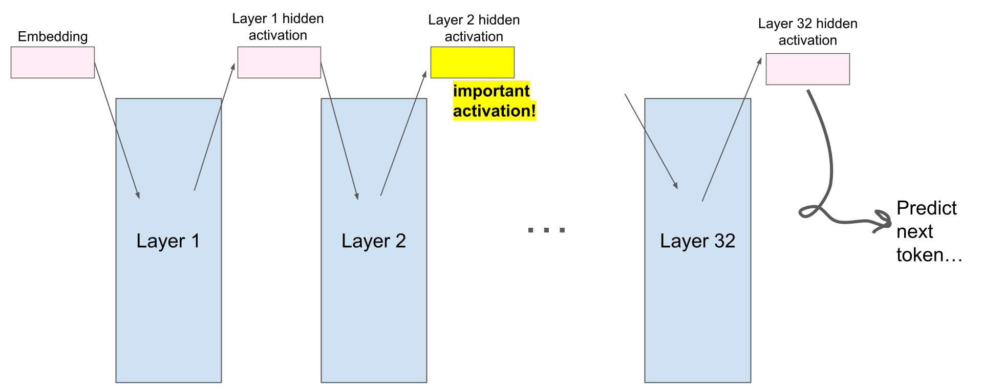
After identifying the influential layers, one can apply their steering vector to just these layers, and ideally, the desired behavior should emerge. This allows us to find the best location for a steering vector without doing a full sweep. And, once again, activation patching requires very few samples to actually deploy. Pretty neat!

Even more localized activation patching

However, activation patching methods don’t end here. Looking at the complex structure of the transformer model, one can see that there are lots of places in the model to perturb and experiment with. Todd et al apply a more specific and localized approach.

Here, the authors want to answer questions about in-context learning. In-context learning (ICL) is when you give the model an example of what you want it to do in the prompt (or, “in-context”). The authors ask, specifically, when the model is given an ICL task, where in its transformer architecture does it store this information?

To answer this question, the authors utilize activation patching. They begin with the more generalized approach from before: first, give a model a set of prompts that have in-context information about a specific task. For each specific layer, average the hidden activations (this is the clean run). Next, give the model a set of prompts relating to a different task. When doing this, at each different layer, inject the activations from the clean run (this is now the corrupted run). If, in doing this, the model still performs the previous task, then this layer is deemed important.

Next, the authors go beyond the layer-level and deploy a more localized approach. They repeat the same process as before, but instead of injecting activations from the clean run at the layer-level, they inject them at the attention-head level. Activations from the discovered influential attention heads are averaged across all prompts for a specific task and used to create a steering vector, or, as the authors call it, a function vector, for this specific task.

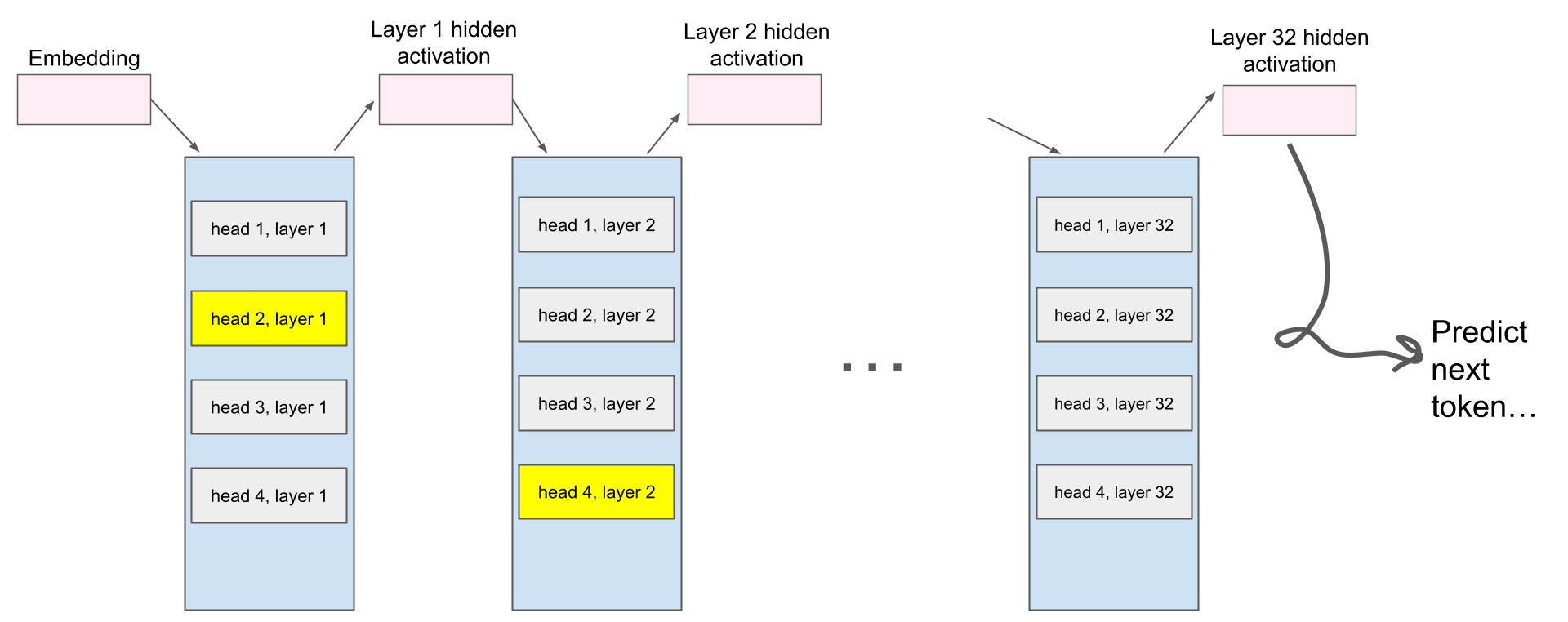
However, as we can see from the structure of the transformer model, every layer has multiple attention heads. If the function vector is created with information from an attention head from Layer 1, and another one from Layer 13, then, at which layer do we apply the finalized function vector? The authors end up conducting a sweep to find the best-performing layer. So, while more fine-grained activation patching may provide a more effective steering vector, it still can require a sweep to find the best location to apply it.

Conclusions

Looking at the transformer architecture, there appears to be an infinite amount of ways that one can edit and perturb the model weights to elicit a desired behavior in a language model. It can oftentimes be more of an art than an exact science. Additionally, representation engineering and mechanistic interpretability as a whole are really unique because they allow us to elicit a model behavior while knowing exactly what is going on ‘inside’ it. RepE concepts don’t only have to be surface-level ones, they can also represent more complex concepts, like truthfulness or function types. Additionally, finding these vectors often requires very little data, which is really useful. I wonder what other types of edits and perturbations can be done to the models, as well as where the limit for the type of information that a steering vector can hold is (if there even is one)!